Chapter 2: Basic Data Manipulation on Time Series

Working with time series data can be intimidating at first. The time series values are not the only information you have to consider. The timestamps also contain information, especially about the relationship between the values. In contrast to common data types, timestamps have a few unique characteristics. While they look like a string at first glance, they also have numerical aspects. This section will present essential techniques for effectively managing time series data.

How to Deal with Datetime Format

The essential part of time series data is the time component. The interval at which the variable or the phenomenon is observed or recorded. In Pandas, they take the form of timestamps. If these timestamps are in Datetime format, you can apply various manipulations, which we will discuss in this section. If not, you will have to convert it into the convenient format to unlock its various functionalities.

Reading Datetime Format

By default, when reading from a CSV file that contains time series, unless carefully coded before hand, Pandas reads timestamp columns as strings into a DataFrame, instead of datetime64[ns] data type. Let’s practice the example below.

import pandas as pd
import matplotlib.pyplot as plt

Example:

Good air quality can have a direct impact on property valuations. For real estate agencies, it is vital to their businesses to study the quality of the air in a certain geographical area before building settlements. The reason is that,

• Areas with better air quality can lead to higher property values.

• Areas with better air quality reduces the risks of respiratory ailments, allergies, and other health problems as Homebuyers and renters often prioritize their health and the health of their families.

• Areas with better air quality tend to have lower maintenance costs. Polluted air can lead to faster wear and tear on building materials, increased cleaning needs, and even damage to property.

Alain-realty, a real estate agency located in Kinshasa, Democratic Republic of Congo, plans to build luxious apartments in response to the improved lifestyle of the Congolese people resulting from the exploitation of coltan mines used in electric cars. They have engaged a team of Engineers from P.L. Global Consulting to assess the air quality in Bagata, an outskirt in Kinshasa. They have installed sensors capable of measuring the Ambiant Temperature, relative and absolute humidity from March 3rd, 2004, to April 4th, 2005, at 30-minute intervals. The resulting data is stored in a csv file provided below.

airqual_data =  pd.read_csv('data/Air_Quality_bagata.csv')
airqual_data

	Date	Temp	Rel_Hum	Abs_Hum
0	2004-10-03 18:00:00	13.6	48.9	0.7578
1	2004-10-03 18:30:00	13.3	47.7	0.7255
2	2004-10-03 19:00:00	11.9	54.0	0.7502
3	2004-10-03 19:30:00	11.0	60.0	0.7867
4	2004-10-03 20:00:00	11.2	59.6	0.7888
...	...	...	...	...
8772	2005-04-04 12:00:00	4.5	56.3	0.4800
8773	2005-04-04 12:30:00	3.8	59.7	0.4839
8774	2005-04-04 13:00:00	4.3	58.6	0.4915
8775	2005-04-04 13:30:00	7.1	50.0	0.5067
8776	2005-04-04 14:00:00	11.1	38.4	0.5066

8777 rows × 4 columns

Let’s explore the data types of each column

airqual_data.info()

<class 'pandas.core.frame.DataFrame'>
RangeIndex: 8777 entries, 0 to 8776
Data columns (total 4 columns):
 #   Column   Non-Null Count  Dtype  
---  ------   --------------  -----  
 0   Date     8777 non-null   object 
 1   Temp     8777 non-null   float64
 2   Rel_Hum  8777 non-null   float64
 3   Abs_Hum  8777 non-null   float64
dtypes: float64(3), object(1)
memory usage: 274.4+ KB

Though the date column contains date instances, its data type is still regarded as an object. Hence , we need to convert into datetime object to use all the date related functionalities. This is done by using the pd.to_datetime() method.

airqual_data['Date']= pd.to_datetime(airqual_data['Date'])
airqual_data.info()

<class 'pandas.core.frame.DataFrame'>
RangeIndex: 8777 entries, 0 to 8776
Data columns (total 4 columns):
 #   Column   Non-Null Count  Dtype         
---  ------   --------------  -----         
 0   Date     8777 non-null   datetime64[ns]
 1   Temp     8777 non-null   float64       
 2   Rel_Hum  8777 non-null   float64       
 3   Abs_Hum  8777 non-null   float64       
dtypes: datetime64[ns](1), float64(3)
memory usage: 274.4 KB

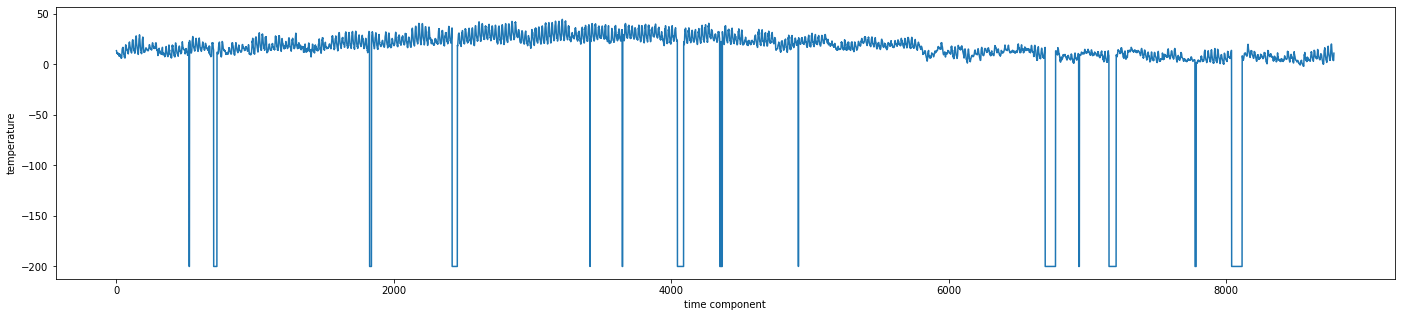
Q:

Let’s get a visual of the series by running the code below to see the evolution of temperature.

1. Report on what you observe?

2. If you have spotted any anomaly, what do you suggest we do about it?

plt.figure(figsize=(24,5))
plt.plot(airqual_data['Temp'])
plt.ylabel('temperature')
plt.xlabel('time component')

Text(0.5, 0, 'time component')

From Datetime to date and time

When you have a date and a timestamp, you can decompose them into their components. As shown below, we are breaking the Date column into actual dates and time column respectively.

# Splitting date and time
airqual_data["dates"] = airqual_data["Date"].dt.date
airqual_data["times"] = airqual_data["Date"].dt.time
airqual_data.head()

	Date	Temp	Rel_Hum	Abs_Hum	dates	times
0	2004-10-03 18:00:00	13.6	48.9	0.7578	2004-10-03	18:00:00
1	2004-10-03 18:30:00	13.3	47.7	0.7255	2004-10-03	18:30:00
2	2004-10-03 19:00:00	11.9	54.0	0.7502	2004-10-03	19:00:00
3	2004-10-03 19:30:00	11.0	60.0	0.7867	2004-10-03	19:30:00
4	2004-10-03 20:00:00	11.2	59.6	0.7888	2004-10-03	20:00:00

Exploring the date

The date itself could also be decomposed it into smaller components, which includes year, month and day as shown below. Further down the line, this could in turn unlock information related to weekly observations, monthly insights or quaterly observations.

airqual_data["year"] = airqual_data["Date"].dt.year

airqual_data["month"] = airqual_data["Date"].dt.month

airqual_data["day"] = airqual_data["Date"].dt.day

airqual_data.head()

	Date	Temp	Rel_Hum	Abs_Hum	dates	times	year	month	day
0	2004-10-03 18:00:00	13.6	48.9	0.7578	2004-10-03	18:00:00	2004	10	3
1	2004-10-03 18:30:00	13.3	47.7	0.7255	2004-10-03	18:30:00	2004	10	3
2	2004-10-03 19:00:00	11.9	54.0	0.7502	2004-10-03	19:00:00	2004	10	3
3	2004-10-03 19:30:00	11.0	60.0	0.7867	2004-10-03	19:30:00	2004	10	3
4	2004-10-03 20:00:00	11.2	59.6	0.7888	2004-10-03	20:00:00	2004	10	3

airqual_data.shape

(8777, 9)

pd.date_range("2021-10-03 18:00:00","2022-04-04 14:00:00", freq='30T')

DatetimeIndex(['2021-10-03 18:00:00', '2021-10-03 18:30:00',
               '2021-10-03 19:00:00', '2021-10-03 19:30:00',
               '2021-10-03 20:00:00', '2021-10-03 20:30:00',
               '2021-10-03 21:00:00', '2021-10-03 21:30:00',
               '2021-10-03 22:00:00', '2021-10-03 22:30:00',
               ...
               '2022-04-04 09:30:00', '2022-04-04 10:00:00',
               '2022-04-04 10:30:00', '2022-04-04 11:00:00',
               '2022-04-04 11:30:00', '2022-04-04 12:00:00',
               '2022-04-04 12:30:00', '2022-04-04 13:00:00',
               '2022-04-04 13:30:00', '2022-04-04 14:00:00'],
              dtype='datetime64[ns]', length=8777, freq='30T')

pd.date_range("2021/01/01", "2021/01/10" , freq='D')

DatetimeIndex(['2021-01-01', '2021-01-02', '2021-01-03', '2021-01-04',
               '2021-01-05', '2021-01-06', '2021-01-07', '2021-01-08',
               '2021-01-09', '2021-01-10'],
              dtype='datetime64[ns]', freq='D')

As you could observe, separate columns have been allocated to year, month and day, which makes it easier to query the data effectively. For instance, see this concrete example.

The first part of the rainy season in the Democratic Republic of Congo usually runs from October to December. Farmers usually termed it as mpisoli ya banzambe (tears of gods). Let’s call it “mpisoli” for the sake of this exercise. Here is how the operations performed above could be useful.

The Enigneers from the P.L. Global Constulting might want to know:

• The maximum air temperature throughout the whole Mpisoli duration,

• The average air temperature of each month of that period.

• The highest absolute humidity for each month of that spell.

Let’s extract those information from the dataframe.

import numpy as np

round(np.random.uniform(14.5, 30.5),1)

28.2

airqual_data.info()

<class 'pandas.core.frame.DataFrame'>
RangeIndex: 8777 entries, 0 to 8776
Data columns (total 9 columns):
 #   Column   Non-Null Count  Dtype         
---  ------   --------------  -----         
 0   Date     8777 non-null   datetime64[ns]
 1   Temp     8777 non-null   float64       
 2   Rel_Hum  8777 non-null   float64       
 3   Abs_Hum  8777 non-null   float64       
 4   dates    8777 non-null   object        
 5   times    8777 non-null   object        
 6   year     8777 non-null   int32         
 7   month    8777 non-null   int32         
 8   day      8777 non-null   int32         
dtypes: datetime64[ns](1), float64(3), int32(3), object(2)
memory usage: 514.4+ KB

airqual_data['month'].unique()

array([10, 11, 12,  1,  2,  3,  4], dtype=int32)

mpisoli_data = airqual_data[airqual_data['month'].isin([10,11,12])]
mpisoli_data

	Date	Temp	Rel_Hum	Abs_Hum	dates	times	year	month	day
0	2004-10-03 18:00:00	13.6	48.9	0.7578	2004-10-03	18:00:00	2004	10	3
1	2004-10-03 18:30:00	13.3	47.7	0.7255	2004-10-03	18:30:00	2004	10	3
2	2004-10-03 19:00:00	11.9	54.0	0.7502	2004-10-03	19:00:00	2004	10	3
3	2004-10-03 19:30:00	11.0	60.0	0.7867	2004-10-03	19:30:00	2004	10	3
4	2004-10-03 20:00:00	11.2	59.6	0.7888	2004-10-03	20:00:00	2004	10	3
...	...	...	...	...	...	...	...	...	...
4279	2004-12-31 21:30:00	27.2	33.3	1.1788	2004-12-31	21:30:00	2004	12	31
4280	2004-12-31 22:00:00	27.5	30.9	1.1155	2004-12-31	22:00:00	2004	12	31
4281	2004-12-31 22:30:00	27.1	33.3	1.1762	2004-12-31	22:30:00	2004	12	31
4282	2004-12-31 23:00:00	26.4	35.1	1.1919	2004-12-31	23:00:00	2004	12	31
4283	2004-12-31 23:30:00	25.6	37.6	1.2131	2004-12-31	23:30:00	2004	12	31

4284 rows × 9 columns

#1. The maximum air temperature throughout the whole Mbula duration

mpisoli_data['Temp'].max()

44.6

#2. The average air temperature of each month of that period.

mpisoli_data.groupby('month')['Temp'].mean()

month
10    11.757891
11    16.026736
12    21.559274
Name: Temp, dtype: float64

#3. The highest absolute humidity for each month of that spell.

mpisoli_data.groupby('month')['Abs_Hum'].max()

month
10    1.4852
11    1.9390
12    2.1806
Name: Abs_Hum, dtype: float64

One could also choose to focus on specific month and get any summary related to that month. See below for instance, the minimum temperature in November 2004.

mpisoli_data[ (mpisoli_data['year'] == 2004) &  (mpisoli_data['month'] == 11)]['Temp'].min() 

-200.0

Strange right?!!

Another interesting insight is that one could also group data in terms of weeks prior to extracting information from it. For the dataframe to respond to the query effectively, we should set the date column as an index of the dataframe using the set_index function.

mpisoli_data.set_index('Date', inplace=True)
mpisoli_data

	Temp	Rel_Hum	Abs_Hum	dates	times	year	month	day
Date
2004-10-03 18:00:00	13.6	48.9	0.7578	2004-10-03	18:00:00	2004	10	3
2004-10-03 18:30:00	13.3	47.7	0.7255	2004-10-03	18:30:00	2004	10	3
2004-10-03 19:00:00	11.9	54.0	0.7502	2004-10-03	19:00:00	2004	10	3
2004-10-03 19:30:00	11.0	60.0	0.7867	2004-10-03	19:30:00	2004	10	3
2004-10-03 20:00:00	11.2	59.6	0.7888	2004-10-03	20:00:00	2004	10	3
...	...	...	...	...	...	...	...	...
2004-12-31 21:30:00	27.2	33.3	1.1788	2004-12-31	21:30:00	2004	12	31
2004-12-31 22:00:00	27.5	30.9	1.1155	2004-12-31	22:00:00	2004	12	31
2004-12-31 22:30:00	27.1	33.3	1.1762	2004-12-31	22:30:00	2004	12	31
2004-12-31 23:00:00	26.4	35.1	1.1919	2004-12-31	23:00:00	2004	12	31
2004-12-31 23:30:00	25.6	37.6	1.2131	2004-12-31	23:30:00	2004	12	31

4284 rows × 8 columns

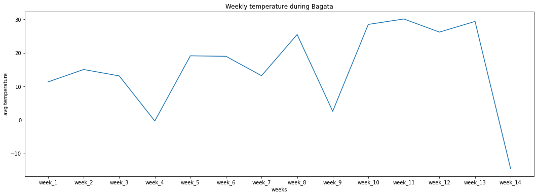
If we are interested in the weekly averages of Temperature or/and absolute humidity during mpisoli, one could groupby the data by weeks using the frequency parameter, and pass in a list of variables we need the aggregates for.

weekly_grouping_mpisoli = mpisoli_data.groupby(pd.Grouper(freq='W'))
mpisoli_data[['Temp', 'Abs_Hum']].mean()

Temp       16.597199
Abs_Hum    -4.902157
dtype: float64

weekly_data_mpisoli = weekly_grouping_mpisoli[['Temp', 'Abs_Hum']].mean().reset_index()

This can lead to answering questions like:

• What is the week with the lowest temperature?

• Does temperature tend to increase on a average on weekly basis or

Or also lead to the generation of weekly summaries as seen below.

weeks = ['week_'+ str(i+1) for i in range(14)]
plt.figure(figsize=(18,6))
plt.plot(weeks, weekly_data_mpisoli['Temp'])
plt.xlabel('weeks')
plt.ylabel('avg temperature')
plt.title('Weekly temperature during Bagata')

Text(0.5, 1.0, 'Weekly temperature during Bagata')

Assembling Multiple Columns to a Datetime

Sometimes, data could be collected in form of separate columns of date components like year, month, and day. We could also assemble that and create a date column from those components still, using the .to_datetime() method. Here, we create a date_2 column to work that out.

airqual_data["date_2"] = pd.to_datetime(airqual_data[["year", "month", "day"]])
airqual_data.head()

	Date	Temp	Rel_Hum	Abs_Hum	dates	times	year	month	day	date_2
0	2004-10-03 18:00:00	13.6	48.9	0.7578	2004-10-03	18:00:00	2004	10	3	2004-10-03
1	2004-10-03 18:30:00	13.3	47.7	0.7255	2004-10-03	18:30:00	2004	10	3	2004-10-03
2	2004-10-03 19:00:00	11.9	54.0	0.7502	2004-10-03	19:00:00	2004	10	3	2004-10-03
3	2004-10-03 19:30:00	11.0	60.0	0.7867	2004-10-03	19:30:00	2004	10	3	2004-10-03
4	2004-10-03 20:00:00	11.2	59.6	0.7888	2004-10-03	20:00:00	2004	10	3	2004-10-03

Task 3:

Monitoring air quality and understanding the data can guide many industries in making informed decisions, adopting cleaner technologies, ensuring public health, and contributing to the overall betterment of the environment. For instance, in Agriculture,

1. Good air quality is necessary for Crop Health, as farmers, could monitor pollutants that can impact crop health and yield.

2. Good air quality could also guide Farming Practices: Selecting crop varieties resistant to certain pollutants or altering farming practices to mitigate the effects of poor air quality.

As a Data Analyst, you are on a working collaboration with JVE Mali, An environmental agency in Mali. The goal is to provide farmers with insights related the Air quality, as this could help them decide whihc plant to grow, when to visit their farms without fearing any respiratory diseases due to air pollution. With the materials acquired from the Government Project titled “Encourger le Paysan Malien (EPM)” which goal is to encourage farming practices among the youth, You have measured different related to polluants in Sikasso

As a Data Analyst, you collaborate with JVE Mali, an environmental agency in Mali. The aim is to provide farmers with insights on Air quality, enabling them to choose suitable crops and also to plan farm regular visits to their plots without respiratory disease concerns. Using materials acquired from the Government Project named “Encourager le Paysan Malien (EPM)” that aims to promote farming practices among young entrepreneurs, JVE have rolled out a data collection campaign across Southern Mali, starting with the City of Sikasso throughout the Year 2022. Some of the polluants’ concentration that were measured include

• PM2.5 (Fine particulate matter)

• PM10 (Coarse particulate matter)

• O₃ (Ozone)

• CO (Carbon monoxide)

• SO₂ (Sulfur dioxide)

• NO₂ (Nitrogen dioxide)

The resulting information is encapsulated in the csv file called sikasso_aq.csv.

1. Load the dataset and tell us what you observe.

2. Produce a dataframe that contains the montly averages of the Coarse particulate matter (PM10). Make sure you replace the month number by the actual month name in your final result. You may use the hint below.

data_frame['month_name'] = pd.to_datetime(data_frame['month'], format='%m').dt.month_name().str.slice()

3. Determine monthly average dynamics of Coarse particulate matter (PM10) and identify the months with lowest and highest average value. Return the results in form of a graph. Save those values somewhere as they represent the \(C_{low}\) and \(C_{high}\) for that polluant.

4. For every other polluant, repeat the Question 2. and 3. above. To avoid re-writing codes from scratch, you might want to customize some functions that perform the Q2 and Q3.

5. Compute the Quaterly average for each of the polluants and report the lowest and largest value for each of the polluants.