Chapter 1: Introduction to Image Data

Introduction

Working with image data offers a myriad of advantages, especially in today’s digital age. At its core, image data provides a rich, multidimensional source of information that can capture intricate details and nuances often missed by other data types.

• Visual Representation and Intuition: Unlike numerical or textual data, images offer a direct visual representation of objects, scenes, and phenomena, allowing for an intuitive understanding and immediate interpretation. This inherent trait of images is especially beneficial in fields like medicine, where radiological images provide direct insights into patient health.

• High Density of Information: Each image can contain millions of pixels, with each pixel holding information about color and intensity, translating to a high data density that’s unparalleled by many other data sources. This information density allows for intricate pattern recognition and fine-grained analyses.

• Versatility across Domains: Image data finds applications in a diverse range of fields - from astronomy, where it aids in exploring distant galaxies, to agriculture, where it helps in assessing crop health using satellite imagery.

Problably, key to this chapter,

• Facilitating Deep Learning and AI: The modern resurgence of neural networks and the success of deep learning are closely tied to image data. Techniques like convolutional neural networks (CNNs) have been primarily nurtured and perfected with image data, achieving feats like real-time object detection, facial recognition, and even artistic style transfers. Temporal Analysis and Evolution Study: Sequences of images captured over time, like time-lapse photography or satellite imagery spanning years, can be invaluable for studying changes, growth, or decay in various contexts, from urban development to environmental changes.

• Augmentation and Enhancement: Image data is malleable. Techniques in image processing can enhance, modify, or even artificially generate images, expanding the possibilities of simulations, entertainment, and even generating training data for machine learning. Empowering Non-Digital Disciplines: Fields that traditionally didn’t rely on digital data, such as archaeology or art history, now leverage image data for digital restorations, 3D reconstructions, or analyzing artistic techniques. In essence, image data, with its richness and ubiquity, not only stands as a cornerstone in the digital information ecosystem but also continuously shapes technological advancements and interdisciplinary innovations.

Learning Objectives:

In this notebook, we’ll explore the basic structure of image data, its significance in the world of machine learning, and learn how to handle and visualize it using common Python libraries.

• Understand the importance and structure of image data.

• Familiarize with common image formats.

• Read and visualize images using Python libraries.

Understanding Image data

In the realm of digital images and deep learning, understanding the mathematical and data structures that represent images is essential. This notebook will walk you through the journey from basic mathematical entities to the complex structures used in image processing.

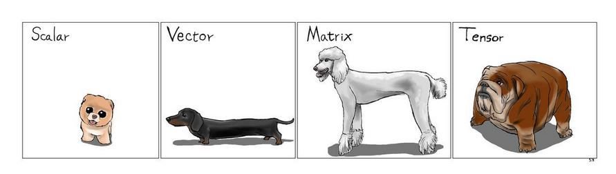
Scalars:

The simplest form of data is a scalar. A scalar is a single numerical value. It doesn’t have direction or multiple dimensions, just magnitude.

scalar = 7
print(f"Scalar Value: {scalar}")

Scalar Value: 7

Vectors

Vectors are one-dimensional arrays of scalars. Think of them as a list of numbers, or in geometric terms, quantities with direction and magnitude.

import numpy as np

vector = np.array([1, 2, 3, 4, 5])
print(f"Vector: {vector}")

Vector: [1 2 3 4 5]

Matrices

A matrix is a two-dimensional array of scalars. If you’ve seen a grayscale image, it can be represented as a matrix, where each entry corresponds to a pixel intensity.

matrix = np.array([[1, 2, 3], [4, 5, 6], [7, 8, 9]])
print(f"Matrix:\n{matrix}")

Matrix:
[[1 2 3]
 [4 5 6]
 [7 8 9]]

Tensors

Tensors can be thought of as multi-dimensional arrays. In the context of images, a colored image is a tensor. It has width, height, and depth (channels - like RGB). So, an RGB image is a 3D tensor.

tensor = np.random.randint(255, size=(4, 4, 3))  # A 4x4 image with 3 channels
print(f"Tensor shape: {tensor.shape}\nTensor:\n{tensor}")

Tensor shape: (4, 4, 3)
Tensor:
[[[197 109 247]
  [ 78  82  66]
  [ 20 168 212]
  [182 177  69]]

 [[190 240 100]
  [145  27 176]
  [ 98  85  39]
  [253 115  46]]

 [[ 32 242 131]
  [ 75  17  48]
  [133 244  84]
  [ 27 144   1]]

 [[151 158 120]
  [ 56 210 219]
  [ 99 109 188]
  [ 73  67 194]]]

from IPython.display import Image

Image('data/scalar_vector_mat_tensor_dogs.jpg')

Understanding Images

A digital image is essentially a tensor. For grayscale images, it’s a matrix, and for colored images with multiple channels (like RGB), it’s a 3D tensor. Each number (scalar) in this tensor represents the intensity of a pixel

import matplotlib.pyplot as plt
sample_image = plt.imread('data/happy_kids_lamu.jpg')
plt.figure(figsize=(8,8))

plt.imshow(sample_image)
plt.title('Sample Image')
plt.axis('off')
plt.show()

print(f"Image shape: {sample_image.shape}")
print(f"Pixel value at (0,0) - RGB: {sample_image[0,0,:]}")

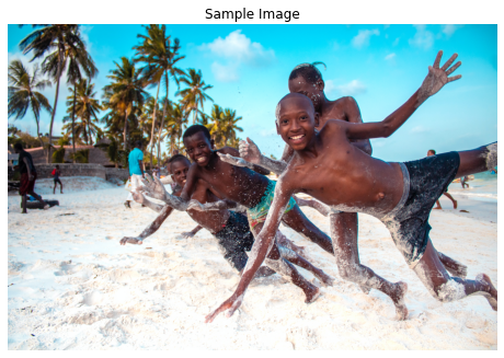
Image shape: (3456, 5184, 3)
Pixel value at (0,0) - RGB: [  1 171 207]

Image Basics

Using OpenCV

# Importing necessary libraries
import numpy as np
import matplotlib.pyplot as plt
import cv2

At its core, an image is just a matrix of pixel values. These pixel values represent the intensity or color information for that pixel.

For grayscale images, this matrix is 2D, where each value represents the intensity of light.

For colored images, typically, we use a 3D matrix, where each ‘layer’ or ‘channel’ of the matrix represents one of the Red, Green, or Blue components of the color (RGB). Some images also come with an additional alpha channel for transparency (RGBA).

Let’s begin by loading an image and exploring its structure.

# Reading an image
image_path = "data/man_fixing_motobike.jpg"  # Replace with the path to your image
image = cv2.imread(image_path)

# Convert from BGR (OpenCV's default) to RGB
image_rgb = cv2.cvtColor(image, cv2.COLOR_BGR2RGB)

# Displaying the image
plt.figure(figsize=(8,8))

plt.imshow(image_rgb)
plt.axis('off')
plt.show()

# Displaying shape and type of the image data
print(f"Shape of the image: {image_rgb.shape}")
print(f"Data type of the image: {image_rgb.dtype}")

Shape of the image: (5184, 3456, 3)
Data type of the image: uint8

Image Formats

There are various image formats available. Some of the common ones include:

• JPEG

• PNG

• BMP

• TIFF

Each format has its own advantages and use cases. For instance, JPEG is commonly used for photographs due to its lossy compression, which reduces file size. PNG, on the other hand, offers lossless compression and supports transparency, making it a popular choice for web graphics.

A TIFF, which stands for Tag Image File Format, is a computer file used to store raster graphics and image information. A favourite among photographers, TIFFs are a handy way to store high-quality images before editing if you want to avoid lossy file formats.

BMP files contain large, raw, high-quality images, which makes them better for editing. They contains uncompressed data, making it ideal for storing and displaying high-quality digital images. On the downside, this lack of compression generally creates larger file sizes than, for example, JPEGs and GIFs

In most machine learning tasks, the exact format is less significant than the underlying pixel values, but it’s still crucial to be aware of the differences, especially when considering image quality and compression.

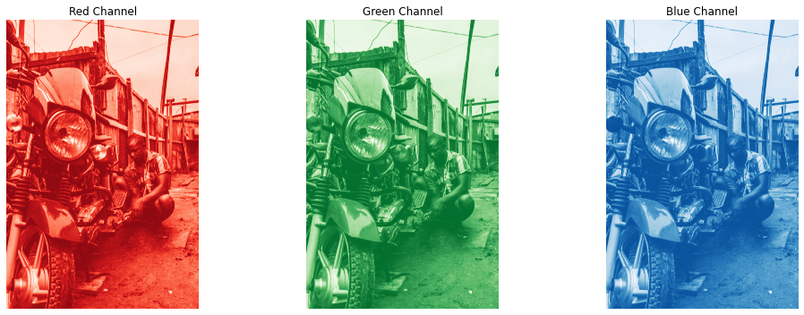
Image Channels

As we observed, our image is represented in the RGB format, which means it has three channels. Let’s visualize each of these channels separately to understand their contribution to the final image.

# Splitting the image into its channels
r, g, b = cv2.split(image_rgb)
list_cols = ['Red', 'Green', 'Blue']
list_channels = ['Reds_r', 'Greens_r', 'Blues_r']
# Displaying each channel
fig, axes = plt.subplots(1, 3, figsize=(15, 5))
for ax, channel, color , chan_ in zip(axes, [r, g, b], list_cols , list_channels):
    ax.imshow(channel, cmap=chan_)
    ax.set_title(f'{color} Channel')
    ax.axis('off')

plt.tight_layout()
plt.show()

Using Tensorflow

import tensorflow as tf
# Load an image using TensorFlow
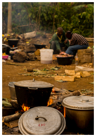
image_path = "data/pot_on_fire.jpg"
image = tf.io.read_file(image_path)
image = tf.image.decode_jpeg(image)

# Display the image
plt.figure(figsize=(8,8))

plt.imshow(image)
plt.axis('off')  # To turn off the axis numbers
plt.show()

Choose 2 images from the data folder.

For each of the images,

• Load it with Opencv and TensorFlow

• Display the different channels as well as their shapes

Task 1: